Virtual Population

Virtual Population

The Virtual Population section creates multiple sets of simulated data, it contains seven sections:

• Scenarios

• Variables

• Correlations

• Advanced Options

• Estimands

• Simulation Options

• Virtual Population Review

Defining the Scenarios

By default, the KerusCloud Virtual Population task will run against one scenario per scenario type, if more than one scenario per type is to be set up, then this should be done prior to defining any variable distributions. Additional scenarios of type Variable, Recruitment, Correlation, Advanced Option and Estimand can be created.

How the number of scenarios are created

KerusCloud creates the combination of scenarios on your behalf to reduce the amount of information you need to enter. Where there are types of scenarios the total number of scenarios is calculated as follows – number of Variable Scenarios x number of Recruitment Scenarios x number of Correlation Scenarios x number of Advanced Option Scenarios x number of Estimand Scenarios. For example if 2 Variable Scenarios, 3 Recruitment Scenarios, 2 Correlation Scenarios, 2 Advanced Option Scenarios, and 3 Estimand Scenarios are defined, then the total number of scenarios will be (2x3x2x2x3) 72.

Simulations can be generated from multiple distributions corresponding to different potential scenarios that might be expected to occur in the “real world”. For example, there may be uncertainty over the variability of a normally distributed variable and hence data may be simulated from a distribution with a low standard deviation as well as from one with a higher standard deviation.

Additional scenarios are set up as follows:

1. Click on the Virtual Population box
2. Click on the Scenarios tab
3. Click the View button for the scenario type
4. Click on the Activate! toggle
5. Click on the + symbol to add more scenarios
6. Give a label to the scenario (no more than 8 characters) and provide an (optional) longer description
7. Click Save
8. Data will be simulated for every scenario independently, so that analyses and the resulting probabilities of success can be assessed and reported separately for each set of simulations corresponding to each scenario

Defining the Variables

A user must enter a name for each variable.

Requirements of a variable name

1. Unique variable names are required per project
2. Variable names must have a minimum length of 1, up to a maximum length of 8.
3. Variable names can only start with a letter
4. Must only include letters, numbers or ‘_’

Data is simulated for each variable using the information provided, by the user, about the distribution and the correlation of the variables with each other.

References can be added to any KerusCloud project. When defining variables there is a bibliography section within the Virtual Population section. Each variable created has a box Refs which can be found next to the View box. This allows the user to link relevant document sources to specific variables. For example, if a scientific article has been used to get estimates for the mean and standard deviation of a variable then the specific information about this article, such as title, author, documentation type can be entered and the entry can be linked to the relevant variable. References can also be linked to any advanced options applied to variables, as well as to correlations.

Variables can be defined as falling into any one of five data types:

1. Special
2. Discrete
3. Continuous
4. Derived
5. Repeated Measures

Which Variables can be used to define subpopulations?

Group, Binomial, Multinomial or Recruitment (recruitment site) variable categories can be used to define subpopulations for which the characteristics of other variables can be defined.

For example, a continuous variable could be defined with different parameter estimates, such as different estimates of variability according to the subgroup levels of a binomial variable. For example, it might be expected that older participants will have a greater variability in response to treatment than younger participants.

Special Data Type

There are three Special variable types: Group, Recruitment and Time-to-Event.

Group

The first is a grouping variable. All other variables and correlations of variables can be defined for separate levels of the Group variable. An example of a Group variable might be treatment with levels placebo and active. It might be relevant to define the distributions of other variables according to the treatment group with a different parameter estimate used in the placebo group to the active treatment group. The Group is also of significance in the allocation section of the Study Design as discussed in Study Design and Analysis section.

Altering the ratio of randomisation between the levels of the Group variable

This is achieved in the Study Design and Analysis.

For example, if Group was defined to have 2 levels: placebo and active treatment, then a 1:1 allocation would generate data with an equal number of samples for each level of group. If an allocation is specified as 2 for active treatment and 1 for placebo, then twice as many samples would be generated for the active treatment group. With a sample size of 90 and a 2:1 allocation then 60 samples would be generated for active treatment and 30 for placebo.

Recruitment

The second type of variable that can be defined in the Special data type is a Recruitment variable. Only one Recruitment variable may be defined per project. At least one Recruitment Site and at least one Recruitment Period must be defined for the Recruitment variable.

For each Recruitment Site and Recruitment Period, a Recruitment Rate must be specified, indicating the rate of recruitment in each case. Specifically, the recruitment rate reflects the average number of subjects recruited per unit time.

For example, consider a study with one Recruitment Site (Site A) and three Recruitment Periods (0-12, 12-24 and 24-Infinity), where each unit of time represents one month. The Recruitment Rate between 0-12 months is 2, meaning on average two subjects will be recruited each month in the first year. Between 12-24 months the Recruitment Rate is 4, meaning an average of four subjects will be recruited to Site A in this period. As a result, it is expected that an average of 72 subjects will be recruited to Site A in the first two years of the study.

Note

The last Recruitment Period always runs until a time of infinity, and cannot have a Recruitment Rate of 0, to ensure that the required sample size is recruited in each simulation.

How to create a recruitment variable

1. Click on the Virtual Population box

2. In the New Variable section enter a name in the Variable Identifier box and a description in the Variable Description box

3. Use the drop-down menu to select Recruitment variable type

4. Recruitment Sites are defined by clicking Customise Recruitment Sites link. At least one recruitment site must be defined. Additional recruitment sites can be added via the ’+’ button. A maximum of ten sites can be defined, Recruitment Site Label must be no more than 8 characters and must be unique. Save Recruitment Sites by clicking Save & Close button

5. Recruitment Periods are defined by clicking Customise Recruitment Periods link. A default recruitment period is defined. Additional recruitment periods can be added via the ’+’ button. A maximum of twelve recruitment periods can be defined, recruitment period upper values must be greater than the upper value of the previous recruitment period. Save Recruitment Periods by clicking Save & Close button

6. Define the Recruitment Rates per Recruitment Period per Recruitment Site by expanding into the Variable Parameters boxes on the right-hand side by clicking on the ’>’ button. Use the ‘Type’ drop-down box to define the values for the recruitment rates per recruitment periods. Entry of the parameter values has the default setting as Single. Click on the down arrow to change the selection to Scenario-based

   a. Single: variable will be simulated for all scenarios from a single distribution defined by the value entered for Recruitment Rates

   b. Scenario-based: variable will be simulated from the distribution defined by the value entered for Recruitment Rates for each Recruitment scenario

7. Click Save

Using a Recruitment variable within an analysis or when defining other variables

If you use a Recruitment variable as a defined by when defining another variable, or as a factor when defining an analysis, the Site aspect of the Recruitment variable is used.

Time-to-Event

Prior to specifying a Time-to-Event variable, two continuous variables must be defined (of type Beta, Exponential, Log-Normal, Uniform or Weibull), representing the event and censoring distribution, respectively. For Time-to-Event outcomes, the data comprises two parts: the first is the follow-up time for each individual, the second is whether they had an event at that time or are right-censored. Click on the Time-to-Event data type, and select which two previously defined continuous distributions will be combined to define the Time-to-Event data: these variables are a Censor Time and an Event Time. KerusCloud will treat all instances where the Event Time is smaller than the Censor Time as an event at the time of the Event Time, and all instances where the Censor Time is smaller than the Event Time as censored at the time of the Censor Time.

Applicable variable types for defining a Time-to-Event variable

All continuous variables with the exception of Normal variables can be used to define a Time-to-Event variable.

How to create a Time-to-Event variable

1. Click on the Virtual Population box
2. In the New Variable section enter a name in the Variable Identifier box and a description in the Variable Description box
3. Use the drop-down menu to select Time-to-Event
4. Click on the Censor Time and use the drop-down to select from one of the previously defined continuous distributions to define the Censor Time
5. Click on the Event Time and use the drop-down to select from one of the previously defined continuous distributions to define the Event Time
6. Click Save

Discrete Data Type

There are four Discrete variable types: Binomial, Multinomial, Negative Binomial and Poisson.

How to create a discrete variable

1. Click on the Virtual Population box
2. In the New Variable section enter a name in the Variable Identifier box and a description in the Variable Description box
3. Use the drop-down menu to select a distribution for the Variable Type

Binomial and Multinomial

A binomial is a discrete distribution with exactly 2 different levels and a multinomial distribution has up to 12 levels with KerusCloud.

How to add details about each level

1. Click on Customise Variable Levels to define each group

   a. Enter a text description into Variable Level Label

   b. Enter a number into the Inferred Value only if the variable is to be used for a numerical purpose at a later stage (eg ordering the categories, or treating them as numeric), otherwise leave empty. See Note 1

   c. To change the order of the Variable Levels, click and drag on the small box to the right of the Variable Level Label box. See Note 2

   d. Click Save & Close

2. Click the Select Option(s) box under the Defined By field to indicate if the values of the variable are defined at a population level or are defined at a subgroup level. The blue box allows the user to search for the subgroup required. Alternatively click on one of the options listed. Up to three subgroups can be selected simultaneously

3. Define the distribution by moving into the Variable Parameter box on the right-hand side and clicking on the “>” to produce drop down fields to enter the probability that a participant will fall into each category

4. Use the drop-down box (under Variable Parameters) to define the distribution for each subgroup/population. Entry of the parameter values has the default setting as Single. Click on the down arrow to change the selection to either Distribution-based or Scenario-based

   a. Single: variable will be simulated for all scenarios from a single distribution defined by the value entered

   b. Distribution-based: the variable parameter will be simulated with the parameter value for each simulation sampled from a distribution of values. This adds uncertainty into the parameter estimates as each observation simulated is based on a parameter that has been randomly selected from a distribution. These distributions can be considered analogous to Bayesian prior distributions for the simulation parameters. Possible distributions to be chosen from are beta, log-normal, normal or uniform

   c. Scenario based: variable will be simulated from the distribution defined by the parameter estimates entered for each scenario

5. Click Save in the upper right corner

Inferred Value

The inferred value assigned to each level is a numeric value that can be used when defining other variables, for example when using the Operational Derivation option.

Level Label

The order of the Variable Level Label is important. The parameter value entered for the proportions defines the rate for the second level. For example, to generate a binomial variable for gender where 70% of the dataset is female and 30% male make sure that the Variable Level Label is “Male” for the second category and then define the parameter value as 0.3. If “Male” is the first category, then the parameter value would refer to “Female” and hence the parameter value would need to be 0.7 to get the correct classification rate. If labels are not defined the default is for the first level to have label “0” and the second level to have value “1” where the parameter value relates to the probability of “1”. Assigning the correct proportion to the correct label is particularly important if the variable is to be used in defining other variables based on these subgroups.

Negative Binomial and Poisson

How to define parameters

1. Click the Select Option(s) box under the Defined By field to indicate if the values of the variable are defined at a population level or are defined at a subgroup level. The blue box allows the user to search for the subgroup required. Alternatively click on one of the options listed. Up to three subgroups can be selected simultaneously

2. Define the distribution by moving into the Variable Parameter box on the right-hand side and clicking on the “>” to produce drop down fields to enter the probability that a participant will fall into each category

3. Use the drop-down box (under Variable Parameters) to define the distribution for each subgroup/ population. Entry of the parameter values has the default setting as Single. Click on the down arrow to change the selection to either Distribution-based or Scenario-based

   a. Single: variable will be simulated for all scenarios from a single distribution defined by the value entered

   b. Distribution-based: the variable parameter will be simulated with the parameter value for each simulation sampled from a distribution of values. This adds uncertainty into the parameter estimates as each observation simulated is based on a parameter that has been randomly selected from a distribution. These distributions can be considered analogous to Bayesian prior distributions for the simulation parameters. Possible distributions to be chosen from are beta, log-normal, normal or uniform

   c. Scenario based: variable will be simulated from the distribution defined by the parameter estimates entered for each scenario

4. Click Save in the upper right corner

Continuous Data Type

The available distribution types of continuous variables are Beta, Exponential, Log-Normal, Normal, Uniform and Weibull.

How to create a continuous variable

1. Click on the Virtual Population box

2. In the New Variable section enter a name in the Variable Identifier box and a description in the Variable Description box

3. Use the drop-down menu to select a distribution for the Variable Type

4. Select Variable Type from the options available

5. Click the Select Option(s) box under the Defined By field to indicate if the values of the variable are defined at a population level or are defined at a subgroup level. The blue box allows the user to search for the subgroup required. Alternatively click on one of the options listed. Up to three subgroups can be selected simultaneously

6. Define the distribution by moving into the Variable Parameter box on the right-hand side and clicking on the “>” to produce drop down fields to enter the parameters that define the distribution for the population/subgroups as appropriate. E.g. for a normal distribution this would be the mean and standard deviation. Entry of the parameter values has the default setting as Single. Click on the down arrow to change the selection to either Distribution-based or Scenario-based

   a. Single: variable will be simulated for all scenarios from a single distribution defined by the value entered

   b. Distribution-based: the variable parameter will be simulated with the parameter value for each simulation sampled from a distribution of values. This adds uncertainty into the parameter estimates as each observation simulated is based on a parameter that has been randomly selected from a distribution. These distributions can be considered analogous to Bayesian prior distributions for the simulation parameters. Possible distributions to be chosen from are beta, log-normal, normal or uniform

   c. Scenario based: variable will be simulated from the distribution defined by the parameter estimates entered for each scenario

7. Click Save in the upper right corner

Derived Data Type

Derived data types allow you to create new variables based on existing variables and can be either Derived Multinomial or Operational Derivation. A Derived Multinomial convert a continuous variable into categories based on cut-points along the distribution and an Operational Derivation applies arithmetic functions to multiple existing variables or constant values.

How to simulate a derived variable

1. Click on the Virtual Population box
2. In the New Variable section enter a name in the Variable Identifier box and a description in the Variable Description
3. Use the drop-down menu to select a distribution for the Derived Variable Type
4. Click Customise

Operational Derivation

How to customise an Operational Derivation

1. If necessary, click on the “+” to add extra rows corresponding to extra levels of derivations required
2. Under function add the required operator
3. Under Input 1 and Input 2 select the variable the derivation will be performed upon or define a value to be used

Derived Multinomial

How to discretize a continuous variable

1. Under Defining variable select the continuous variable to be used to define categories
2. Clink on the “+” to add extra rows corresponding to different numbers of cut-points for different categories
3. Under Value enter the value of the first cut-point
4. If multiple cut-points are required then continue to add the value of each cut-point
5. Under Variable Level Label write a description for each category

Inheriting Advanced Options

The Inherit Advanced Options is selected by default to ensure that any selected on the chosen continuous variable are maintained in the created categorical variable. This can be deselected if necessary.

Repeated Measures Data Type

Repeated Measures (RM) variables can be created in KerusCloud to represent observations of the same variable across multiple study Timepoints. There are three available repeated measures data types: Continuous RM, Irreversible Event and Reversible Event. Continuous RM and Reversible Event variables can only be created when a project has at least one variable of a valid type (see below).

How to create a Repeated Measures variable

1. Click on the Virtual Population box
2. In the New Variable section enter a name in the Variable Identifier box and optionally a description in the Variable Description
3. Use the Variable Type menu to select one of the Repeated Measures types
4. Enter the required details for the selected variable type (described in detail below)
5. Click Save in the upper right corner

Continuous RM

Continuous RM variables represent repeated observations of a variable at multiple Timepoints. For example, blood pressure measured at 0, 4 and 8 weeks. Before creating a Continuous RM variable, separate variables must be created to represent data at each timepoint. Valid variable distributions for the timepoint variables are all continuous distributions as well as Poisson, Negative Binomial, and Binomial or Multinomial distributions with inferred values.

To enter the details required for a Continuous RM variable

1. Under Variable Parameters, select a variable by clicking in the Available Variables list and clicking the > button to move the variable to the Selected Variables list. Selected variables can be moved back to the Available Variables list by selecting and clicking the < button
2. A minimum of 2 timepoint-defined variables are required. A maximum of 12 timepoint-defined variables may be selected. Only one variable may be moved at a time
3. Only valid variable types will be available for selection in the Available Variables list
4. If multiple Available Variables are defined at the same timepoint, selecting one of these will move that variable to the Selected Variables list, the other variables defined at the same timepoint will no longer be listed in Available Variables

Irreversible Event

Irreversible Event variables simulate whether an event has occurred by specific Timepoints. Irreversible means that if the event has occurred for a participant at a given timepoint, the event must also have occurred for that participant at all following timepoints. An example of an irreversible event could be the participant leaving the study. Irreversible Event variables are defined by specifying a set of Timepoint and Probability that the event for a participant has occurred by each time.

How to create an Irreversible Event

1. Clicking Customise Timepoints allows Variable Timepoints to be defined for the Irreversible Event variable. Variable Timepoints must be positive numeric values, unique and in ascending order

2. A minimum of 2 timepoints are required. Timepoints can be added using the + buttons. If a variable has at least 3 timepoints it is possible to remove a timepoint using the - buttons. A maximum of 12 timepoints may be defined

3. Select Single or Scenario-based for the Type next to each Timepoint

   a. Single: Enter a value between 0 and 1 in the Probability box to represent the probability that the event has occurred by the associated time

   b. Scenario-based: Enter values between 0 and 1 in the Probability boxes for each variable scenario to represent the probability that the event has occurred by the associated time for the given scenario

4. The probability values entered must be strictly increasing with time within each scenario

5. To label the event status for each participant click Customise Levels

   a. In the first Variable Level Label box enter a label to indicate that an event has not occurred. By default, this label is “0”

   b. In the second Variable Level Label box enter a label to indicate that an event has occurred. By default, this label is “1”

   c. The level labels can be swapped by dragging to re-order

Reversible Event

Reversible Event variables simulate the status of an event at specific Timepoints. Reversible means that it is possible for an event status to change in either direction between timepoints. For example, a participant could be positive for an event at timepoint 1, negative at timepoint 2 and positive again at timepoint 3. Reversible Event variables are defined using Binomial variables to represent whether the event has occurred at each timepoint. Before creating a Reversible Event variable, Binomial variables must be created to simulate the data for each timepoint. Note that it is not necessary for the level labels of the Binomial variables to be consistent – the first level of each Binomial is treated as the event not occurring and the second level as the event occurring irrespective of the Binomial variable level labels.

How to create a Reversible Event variable

1. Under Variable Parameters, select a variable by clicking in the Available Variables list and clicking the > button to move the variable to the Selected Variables list. Selected variables can be moved back to the Available Variables list by selecting and clicking the < button

2. A minimum of 2 timepoint-defined variables are required. A maximum of 12 timepoint-defined variables may be selected. Only one variable may be moved at a time

3. Only valid variable types will be available for selection in the Available Variables list

4. If multiple Available Variables are defined at the same timepoint, selecting one of these will move that variable to the Selected Variables list, the other variables defined at the same timepoint will no longer be listed in Available Variables

5. To label the event status for each participant click Customise Variable Levels

   a. In the first Variable Level Label box enter a label to indicate that an event has not occurred. By default, this label is “0”

   b. In the second Variable Level Label box enter a label to indicate that an event has occurred. By default, this label is “1”

   c. The level labels can be swapped by dragging to re-order

Tip

The available variables must have a timepoint attribute assigned to them and must be different from existing constituent variables.

Cascading Deletion

Deleting a variable that is a component of a Repeated Measures variable will also delete the Repeated Measures variable.

Timepoints

Timepoint is an optional attribute that can be added to variable(s) that indicate how much time has elapsed since the start of the trial to when the data was obtained. Timepoints are entered in arbitrary units to provide maximum flexibility and accommodate trials with different timescales to variables.

Note

When entering a timepoint, it is assumed to be from the perspective of the patient. If a project has a recruitment variable, then not all patients will be recruited at the start of the trial.

An optional timepoint attribute, that can be provided to Continuous and Discrete variables, is entered as a single positive numeric value under the Variable Timepoint field. Where a variable that is defined by additional variable(s), the original variable timepoint is used. Although the Defined By variable(s) may have been obtained at a later timepoint, it is assumed that this underlying information existed but hadn’t been measured at that timepoint.

Time of Group variable

For a Group variable the timepoint is added as an implicit assumption of KerusCloud as this information is available at the start of the trial – i.e. a timepoint of 0.

Timepoint of Derived variables

For Derived variables, the timepoint is the maximum timepoint of all constituent variables, as this is the timepoint at which all information is available. If a Derived variable has no constituent variable(s) then this is assumed to be timepoint of 0. For example, it would be assumed you have all constants available at timepoint 0.

Timepoint of Time-to-Event variables

In KerusCloud, Time-to-Event variables consist of the time distribution and the Event/Censored label for each participant. However, the overall timepoint of Time-to-Event variable is assumed to be 0 to enable integration of Time-to-Event variables with other variables which may or may not have an associated timepoint.

An Irreversible Event has an optional entry box for assigning multiple interim timepoint(s). These must be a unique positive numeric value in ascending order. Although the Defined By variable(s) may have been obtained at a later timepoint, it is assumed that this underlying information existed but hadn’t been measured at that timepoint.

Timepoint Units

KerusCloud allows timepoint values to be entered in any unit of time to provide maximum flexibility. It is important that all timepoint entries are entered in the same unit of time You can note which time unit you use within the Project Description or Variable Description fields for future reference.

Correlations

Correlations can be defined between any pair of continuous or discrete variables. Three types are available: Pearson R, Spearman Rho and Kendall Tau. Details of how data is simulated under the defined correlation structure . Correlations can be defined at a population level, a group level if a group variable was created, or defined by multiple binomial or multinomial variables.

How is a correlation matrix generated in KerusCloud?

KerusCloud generates a correlation matrix for the Virtual Population with the desired marginal distributions and correlations following these steps:

1. Utilise specially developed in-house models to recalibrate the initial correlations. This ensures the post-copula correlations between the non-normal variables are as required.
2. Simulate correlated multivariate normal data.
3. Transform data using copulas to obtain the desired marginal distribution for each variable.
4. Add advanced options such as missing data, censoring, etc.
5. Check the accuracy of the procedure through built-in quality checks to confirm that the simulated data are sufficiently close to the initially requested inputs.

Advanced Options

To add advanced options to any variable, click on the View tab next to the variable. Valid options are displayed in the right-hand panel according to what is suitable for the distribution. All available options will be displayed in white boxes. Any option box that is selected will turn blue and a sub box will appear below showing that the advanced option has been selected. Clicking on the sub box allows parameters to be specified for inputs. Multiple options can be selected for each variable. For example, Accuracy and Missingness can both be applied to a binomial variable. The order in which the options are applied to the variable can be adjusted by clicking and dragging on the small square on the right of the sub box.

To remove any option simply click on the relevant option box which should return the colour of the box to white to show that it has been removed and then click Save in the top right of the Virtual Population section.

No advanced options can be defined for any Group or Derived type variable.

Inheriting Advanced Options

Derived variables inherit advanced options from the variables from which they are derived

Missingness

All data types except for the Group and Derived Type can have a value for Missingness assigned. Within the Advanced Options tab click on the variable to be adapted, then click on the Missingness tab and define which level to incur the missingness. If at the population level, then just one value is entered which gives the percentage of missing data to be generated across the whole population. If it is anticipated that there will be more missing data within a particular group, then a percentage can be entered for each level of the group.

Note

A Derived Type will have missingness carried over from the variables that the derivation is performed upon but missingness cannot be applied after creation of the derived variable.

Accuracy

Any variables created under the binomial distribution can have an Accuracy value assigned. This allows a percentage value to be entered for sensitivity and specificity. Click on the Accuracy tab.

Note

Percentage values can only be entered at the population level. Inputting a sensitivity value of x randomly converts (100 – x)% of the simulated “successes” for the variable to “failures” after advanced options are applied, where a failure corresponds to the first level of the binomial (with default label “0”) and a success to the second label of the binomial (with default label “1”). A specificity value of y randomly converts (100 – y)% of the simulated “failures” to “successes” after advanced options are applied.

Truncation

Any variables created under the Continuous Data Type or a negative binomial or poisson distribution can have an Upper Truncation or Lower Truncation or both assigned. Click the Lower or Upper Truncation box, then click on the Select Option(s) box under the Defined By field to indicate if the values of the truncation are defined at a population level or are defined at a subgroup level. Entry of the parameter values has the default setting as Single. Click on the down arrow to change the selection to Scenario-based so that different truncation levels can be applied to different scenarios. The truncation procedure has 2 options:

1. Missing which will set all values that fall under the Lower Truncation value or above the Upper Truncation value to missing.
2. Replacement Value which will replace any value that falls above the Upper Truncation value or below the Lower Truncation value to the specified replacement value.

Imputation

An Imputation advanced option can be added for any Continuous or Discrete Data Type and can be applied at a population level or be defined at a subgroup level by changing the Defined By option. The default Impute with option is Single, and this can be changed to Scenario-based to use a different imputation procedure in each advanced option scenario. Imputation replaces any missing variable values with a user-specified value if the Value option is selected, or a value calculated from the non-missing values if one of the Mean, Median, Minimum or Maximum summary options is selected. The summary options are only available for Binomial or Multinomial options with Inferred Values and the inferred values will be used for calculating the replacement value for these distributions. Both user-specified and calculated numeric replacement values are rounded to the nearest “allowed” value for the distribution type. For example, replacement values will be rounded to non-negative integers for a Poisson distribution and positive numbers for a Log-Normal distribution. When selecting the Value option for a Binomial or Multinomial distribution the user will be able to choose one of the level labels to use as a replacement value. Missing values will not be replaced when the None option is selected. This option can be used to explore advanced option scenarios with and without Imputation. Please note that advanced options for each variable are applied in the order they are defined so Imputation must be applied after Missingness or Truncation for it to replace missing values.

Digits

Any variables defined as Continuous Data Types can have a value for Digits assigned to them. Click on Digits, then click on the function to be applied. The default option is Single. This option applies the same procedure to every value. If this is changed to Scenario-based then a separate procedure can be applied to each scenario.

Digits: Round

An integer value between -3 and 7 can be entered for the Round value. The value entered uses the position relative to the decimal point to determine the level of rounding. For example, an entry of -2 rounds the value to the nearest hundred (this being the position that is two places to the left of the decimal point). An entry of 1 rounds the value to one decimal place (this being the position that is 1 place to the right of the decimal point).

Note

KerusCloud uses a round-to-even methodology to reduce bias and as the IEEE standard method for rounding.

Table illustrating how the rounding works for a value of 3456.7804

Level of rounding	None	-2	-1	0	1	2	3	4	5
Resulting number	3456.7804	3500	3460	3457	3456.8	3456.78	3456.780	3456.7804	3456.7804

Digits: Significant

An integer value between 1 and 7 can be entered for the Significant value. This will round simulated data values to the specified number of significant digits.

Table illustrating how rounding with significant figures operates.

Level of rounding	None	1	2	3	4	5
Value 1	3456.7804	3000	3500	3460	3457	3456.8
Value 2	0.001008	0.001	0.001	0.00101	0.001008	0.001008
Value 3	12.3006	10	12	12.3	12.30	12.301

Estimands

The Estimands section of the Virtual Population allows the user to define estimands describing how data should be handled in different situations. For example, if a study participant stopped taking their medication. Estimands in KerusCloud are created in two stages, described in more detail below. Firstly, one or more Estimand Conditions must be defined. Next, Estimand Intercurrent Event Strategies are defined, which are applied to a variable based on the result of a selected Estimand Condition.

Note

Estimands are calculated after Advanced Options have been applied to each variable. Analyses are evaluated after Estimands have been applied to each variable.

Estimand Conditions

Estimand Conditions represent intercurrent events and are used to restrict the subgroup of participants to which an Estimand Intercurrent Event Strategy is applied.

Within the Estimands section, select Customise Conditions to create, view or edit a project’s Estimand Conditions. Each condition must have a label which is used to select that condition when defining Estimand Intercurrent Event Strategies. A description can also optionally be provided.

There are two types of Estimand Condition: Single and Combined.

Single Estimand Conditions compare a variable against one of the following:

• a user-specified value (when Value is selected)

• missingness (when Missing is selected)

• another variable (when Variable is selected)

For Variable-to-Value comparisons, Continuous, Negative Binomial, Poisson, Operational Derivation, Continuous Repeated Measure and Time-to-Event variables can be compared with a numeric value entered by the user. Group, Binomial, Multinomial, Derived Multinomial, Irreversible Event and Reversible Event variables require a variable level label to be selected from the Variable Level dropdown menu.

For Variable-to-Missing comparisons, variables are checked for missingness, which is defined as an Advanced Option.

For Variable-to-Variable comparisons, variables of the following type can be compared with each other: Continuous, Negative Binomial, Poisson, Operational Derivation, Continuous RM and Time-to-Event. Similarly, categorical variables of the following type can be compared: Binomial, Multinomial, Derived Multinomial, Irreversible Event and Reversible Event.

Note

Only the “Time” aspect of Time-to-Event variables is considered when evaluating an Estimand Condition.

Comparison logic options specify the exact comparison evaluated by each condition. E.g. the result of condition “VarX != Missing” will be True for all participants where variable “VarX” is not missing. Similarly, the result of condition “VarY < Value: 5” will be True for participants that have a value less than 5 for variable “VarY”.

Note

Estimand Conditions are evaluated based on the variable data after Advanced Options have been applied, but before Estimands have been applied.

Combined Estimand Conditions can be created when at least two Single Estimand Conditions have been defined, combing the outcome of two estimand conditions for each participant using AND or OR logic. Combined conditions can be defined using Single or Combined conditions, enabling complex situations to be captured based on the result of multiple individual conditions.

Variable Timepoints and Estimand Conditions

Variable timepoints are considered when each Estimand Condition is evaluated. Variables and Values which do not have Timepoints are considered as remaining constant across the study, with an effective timepoint of 0. This includes Time-to-Event variables, as time is inherent for this variable type. These timepoints are compared and condition results generated for matching timepoints. Similarly, when evaluating Variable-to-Variable Estimand Conditions, variable timepoints are compared and condition results generated for each matching timepoint. Where timepoints do not match exactly, the Left Hand Side and Right Hand Side of the condition are compared based on the “most recent” data, where available.

Example: Variable-to-Value Estimand Condition

For example, if a variable with timepoint 1 is compared with a value with an assumed timepoint of 0, the estimand condition will be evaluated at each of these timepoints. However, the condition result for each participant at timepoint 0 will be False, as data is not available at this time for the second variable.

Condition 1: VarA (Timepoint = 1) vs Value (Timepoint = 0)

Results at timepoint: 0 = False, 1 = True/False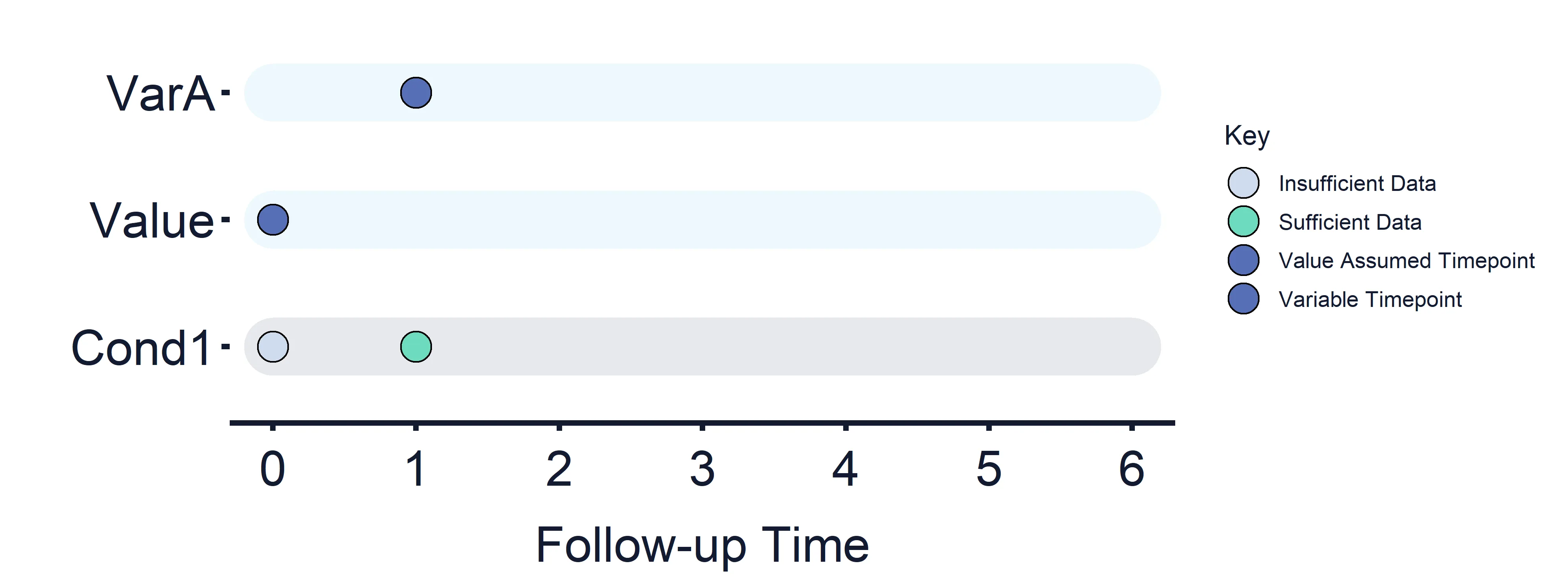

Figure 2: Variables and Estimand Conditions timeline. Condition 1.

Example: Variable-to-Value Estimand Condition with Repeated Measures

For example, if a Repeated Measures variable with timepoints 2, 3, 5 is compared with a value with an assumed timepoint of 0, the estimand condition will be evaluated at each of these timepoints. However, the condition result for each participant at timepoint 0 will be False, as data is not available at this time for the second variable.

Condition 2: VarB (Timepoints = 2, 3, 5) vs Value (Timepoint = 0)

Results at timepoint: 0 = False, 2, 3 and 5 = True/False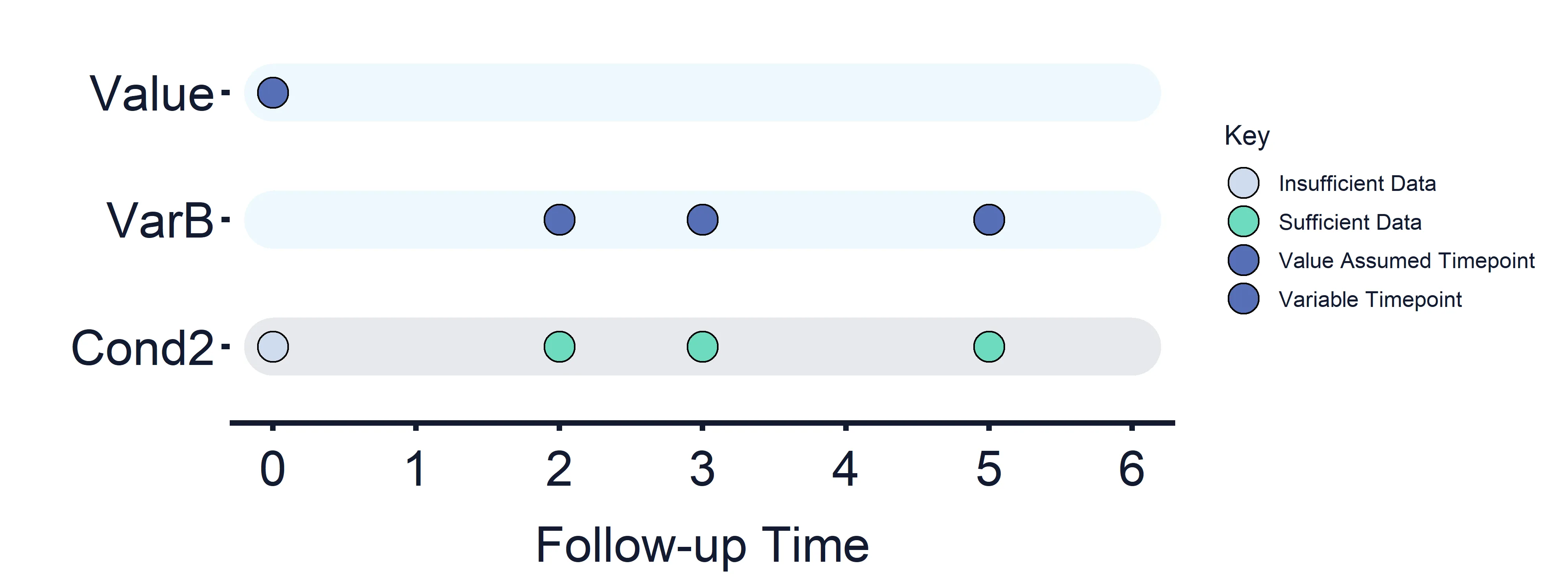

Figure 3: Variables and Estimand Conditions timeline. Condition 2.

Example: Combined Estimand Condition

The results of a Combined Estimand Condition comparing Estimand Condition 1 and 2 defined above would have the following timepoints: 0, 1, 2, 3 and 5. However, the condition result at each timepoint would depend on the timepoints of Condition 1 and Condition 2 results, and the type of logic used to combine these results.

In this example, the condition results at time 0 would always be False, based on the logic described in previous examples.

When AND logic is used, the condition result for each participant at timepoints 2, 3 and 5 would be True, based on the behaviour described above. The condition results at timepoint 1 would be False, as there are no condition results for Condition 2 at this timepoint.

When OR logic is used, the condition result at timepoint 1 would be dictated by the results of Condition 1, as the result of Condition 2 for each participant at this timepoint would be False, as data is only available for one of the variables compared in this condition at these timepoints.

The condition result for each participant at timepoints 2, 3 and 5 would depend on the results of both conditions, regardless of the logic used, as all variables compared in each condition have data at this timepoint.

AND Logic:

Combined Condition 1 AND: Condition 1 (Timepoints = 0 (False) and 1) AND Condition 2 (Timepoints = 0 (False), 2, 3, 5)

Results at timepoint: 0 = False, 1 = False, 2 = True/False, 3 = True/False, 5 = True/False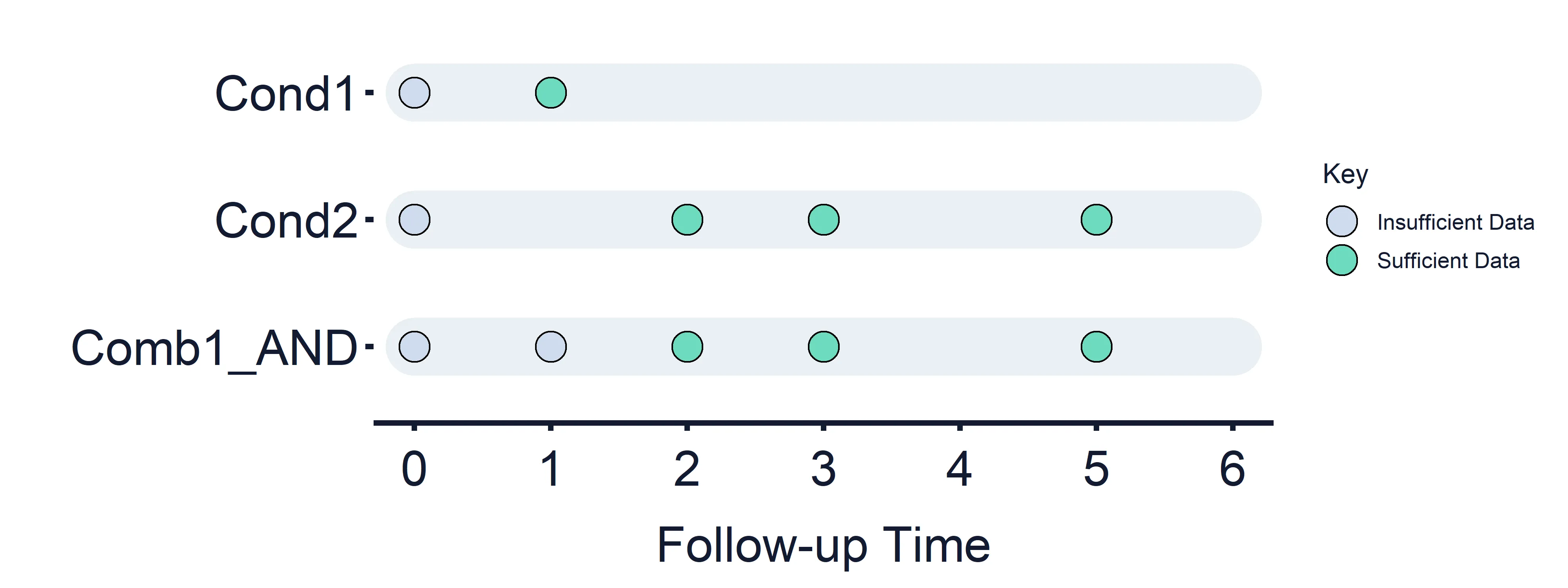

Figure 4: Combined Estimand Conditions timeline. Combined Condition 1 AND logic.

OR Logic:

Combined Condition 1 OR: Condition 1 (Timepoints = 0 (False) and 1) OR Condition 2 (Timepoints = 0 (False), 2, 3, 5)

Results at timepoint: 0 = False, 1 = True/False dependent on the results of Condition 1, 2 = True/False, 3 = True/False, 5 = True/False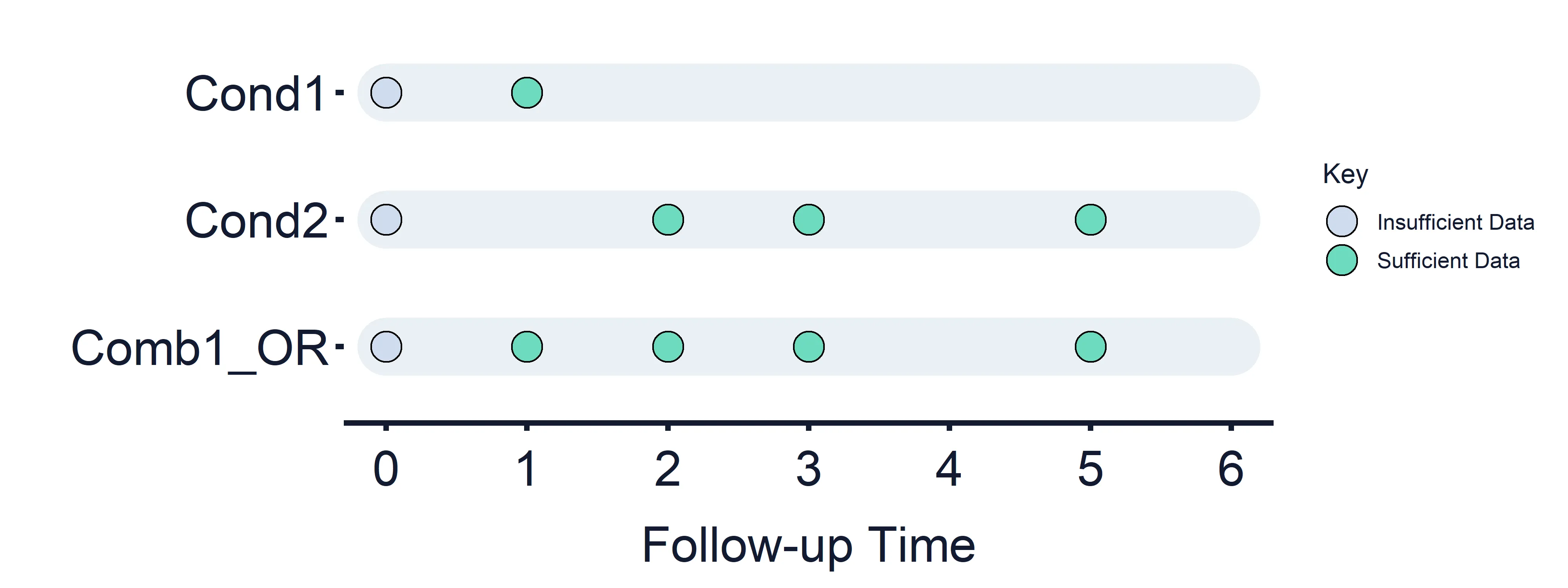

Figure 5: Combined Estimand Conditions timeline. Combined Condition 5 OR logic.

Example: Variable-to-Variable Estimand Condition

For example, if two variables are compared with timepoints 1 and 6 respectively, the estimand condition will be evaluated at each of these timepoints. However, the condition result for each participant at timepoint 1 will be False, as data is not available at this time for the second variable.

Condition 3: VarA (Timepoint = 1) vs VarB (Timepoint = 6)

Results at timepoint: 1 = False, 6 = True/False

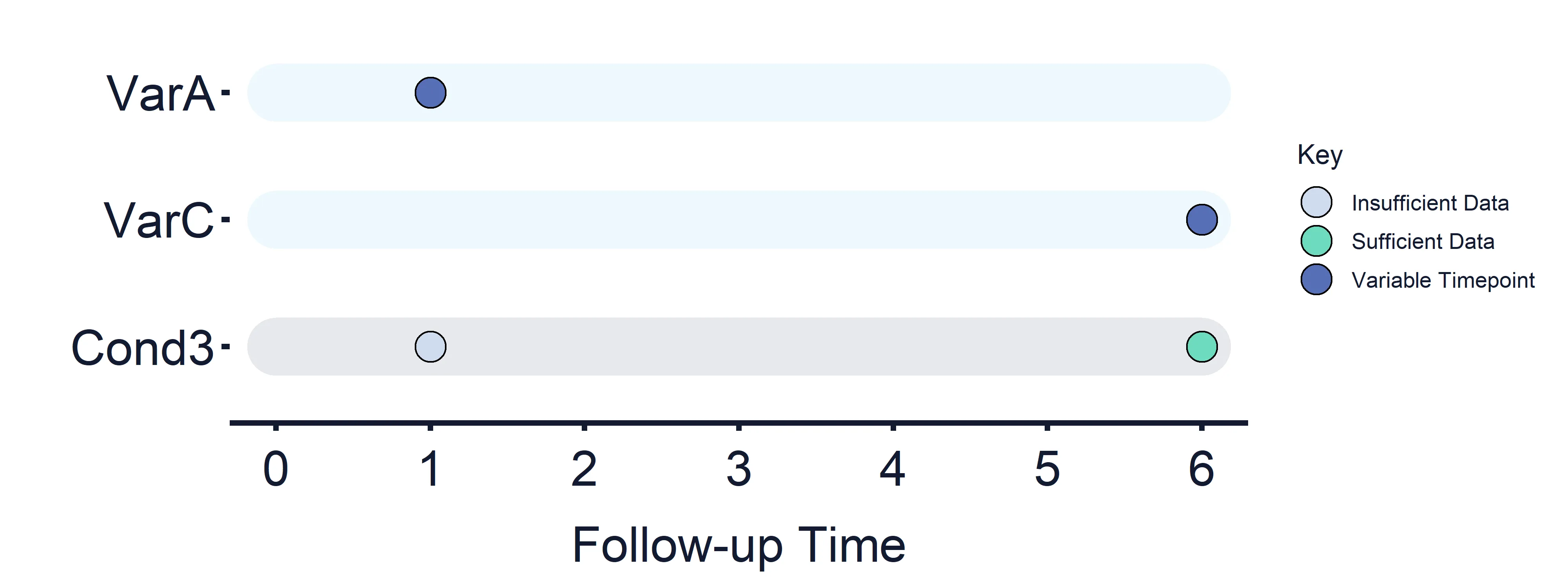Figure 6: Variables and Estimand Conditions timeline. Condition 3.

Example: Variable-to-Variable Estimand Condition with Repeated Measures

Similarly, if a Repeated Measures variable with timepoints 2, 3 and 5 is compared with a variable with a timepoint of 4, the estimand condition will be evaluated at each of these timepoints. However, the condition result for each participant at timepoints 2 and 3 will be False, as data is not available for the second variable at these times.

Condition 4: VarC (Timepoints = 2, 3, 5) vs VarD (Timepoint = 4)

Results at timepoint: 2 = False, 3 = False, 4 = True/False, 5 = True/False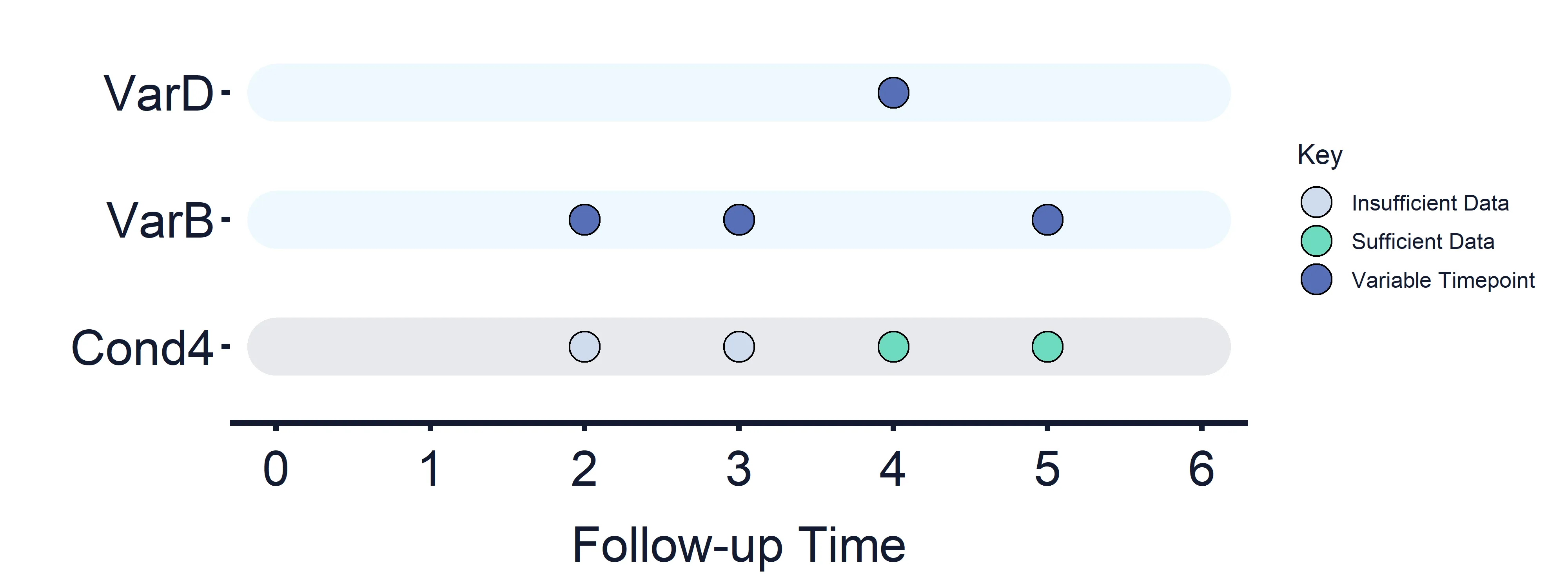

Figure 7: Variables and Estimand Conditions timeline. Condition 4.

Example: Combined Estimand Condition based on Variable-to-Variable comparisons

The results of a Combined Estimand Condition comparing Estimand Condition 3 and 4 defined above would have the following timepoints: 1, 2, 3, 4, 5 and 6. However, the condition result for each participant at timepoints 1, 2 and 3 would be False, based on behaviour described above. When AND logic is used, the condition result for each participant at timepoints 4 and 5 would be False, based on the behaviour described above. When OR logic is used, the condition result at timepoints 4 and 5 would be dictated by the results of Condition 4, as the result of Condition 3 for each participant at these timepoints would be False, as data is only available for one of the variables compared in this condition at these timepoints. The condition result for each participant at timepoint 6 would depend on the results of both conditions, regardless of the logic used, as all variables compared in each condition have data at this timepoint.

AND Logic:

Combined Condition 2 AND: Condition 3 (Timepoints = 1 (False) and 6) AND Condition 4 (Timepoints = 2 (False), 3 (False), 4 and 5)

Results at timepoint: 1 = False, 2 = False, 3 = False, 4 = False, 5 = False, 6 = True/False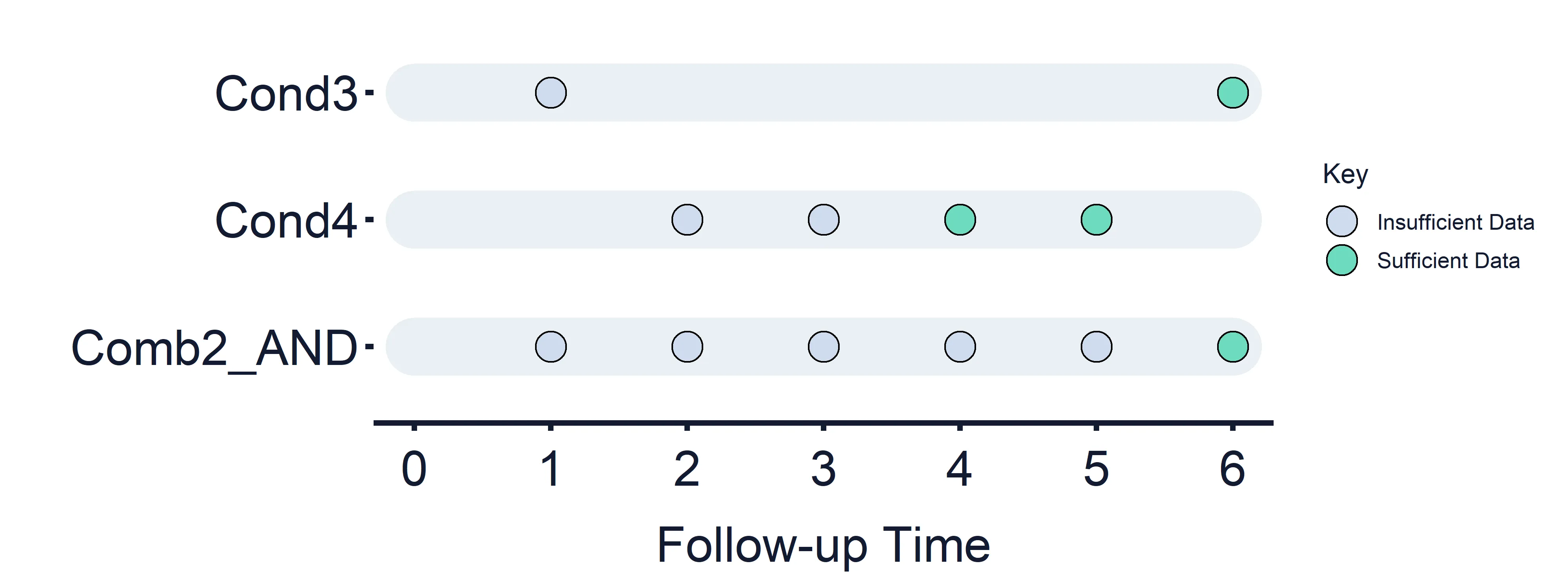

Figure 8: Combined Estimand Conditions timeline. Combined Condition 2 AND logic.

OR Logic:

Combined Condition 2 OR: Condition 3 (Timepoints = 1 and 6) OR Condition 4 (Timepoints = 2, 3, 4 and 5)

Results at timepoint: 1 = False, 2 = False, 3 = False, 4 = True/False dependent on the results of Condition 2, 5 = True/False dependent on the results of Condition 2, 6 = True/False.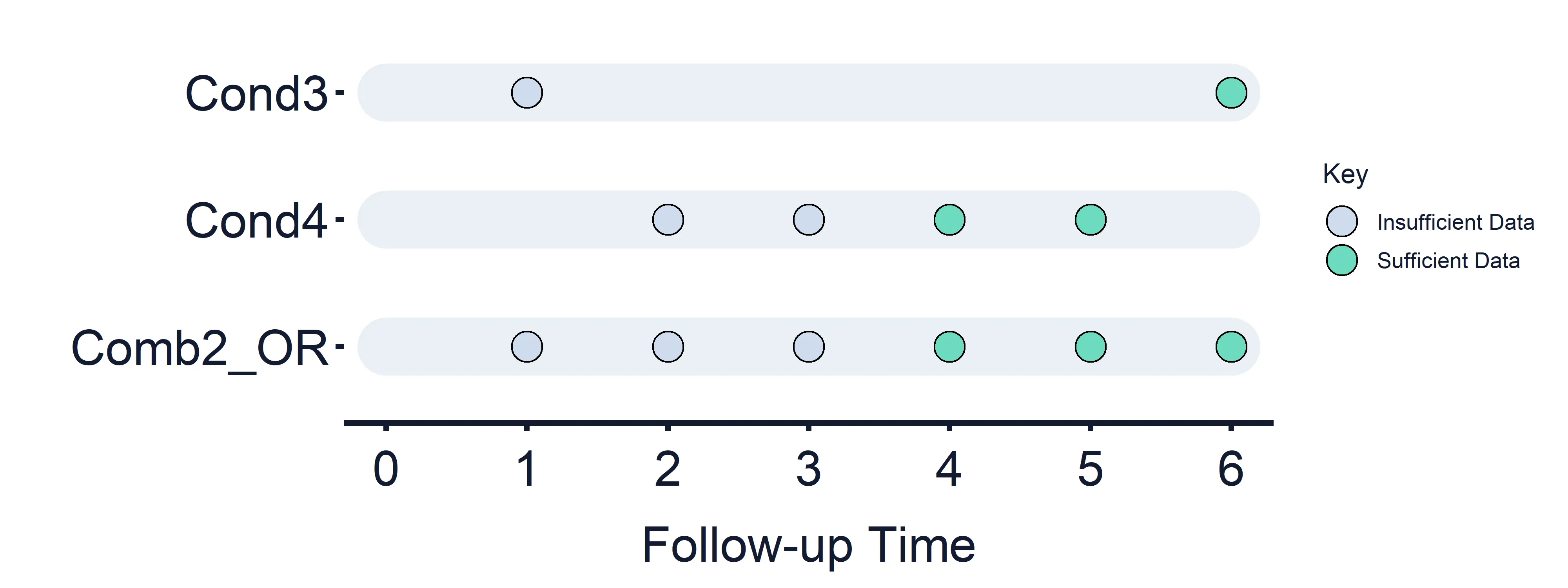

Figure 9: Combined Estimand Conditions timeline. Combined Condition 5 OR logic.

Each Estimand Condition result therefore has an associated timepoint or set of timepoints, including Variable-to-Value, Variable-to-Missing, Variable-to-Variable and Combined estimand conditions.

Estimand Intercurrent Event Strategies

Estimand Intercurrent Event Strategies describe how variable data should be handled in the case of intercurrent events (captured by Estimand Condition results).

To view, create and edit Estimand Intercurrent Event Strategies for a specific variable, select View beside that variable within the Estimand variable table. Variables can have a maximum of one Estimand Definition, composed of one or more Intercurrent Events which are defined based on the result of an estimand condition and the desired estimand replacement strategy.Estimand Intercurrent Event Strategies can be added or removed using the “+” or “-” icons. Up to 12 Intercurrent Events can be created for each variable.

For each Intercurrent Event, when the Estimand Condition (selected using the ‘Condition’ dropdown) is evaluated to True for a participant, the value of the variable for that participant will be updated according to the specified Estimand Strategy. If more than one Intercurrent Event is defined, they will be evaluated in ascending numerical order.

Note

The order Intercurrent Events are defined in is important. For each participant, only the first Intercurrent Event where the condition is evaluated to True will be used to replace the variable value for each participant. Subsequent Intercurrent Events are only considered for that participant if none of the previous Intercurrent Event conditions have been evaluated to True, or if the “No Change” replacement strategy has been selected as the Estimand Intercurrent Event Strategy (described in more detail below).

 

Variable Timepoints and Estimand Intercurrent Event Strategies

In each case, Estimand Condition result Timepoints are compared against the timepoint(s) of the target variable for which the estimand is defined. Condition results with a timepoint matching that of the target variable are used to inform whether the Estimand Strategy is applied to that variable for each participant. Where available, the “most recent” condition results are used when there are no matching timepoints between the condition results and target variable.

Example: Applying an Estimand Strategy where Variable Timepoints have been used

For example, if an estimand is defined for a variable with timepoint = 1 based on the results of Condition 2 (defined above), the results of condition 2 at timepoint 0 are used. In this example, as data is only available for one side of the comparison defined in Condition 2 at timepoint 0, all condition results will be False and no estimand strategy will be applied.

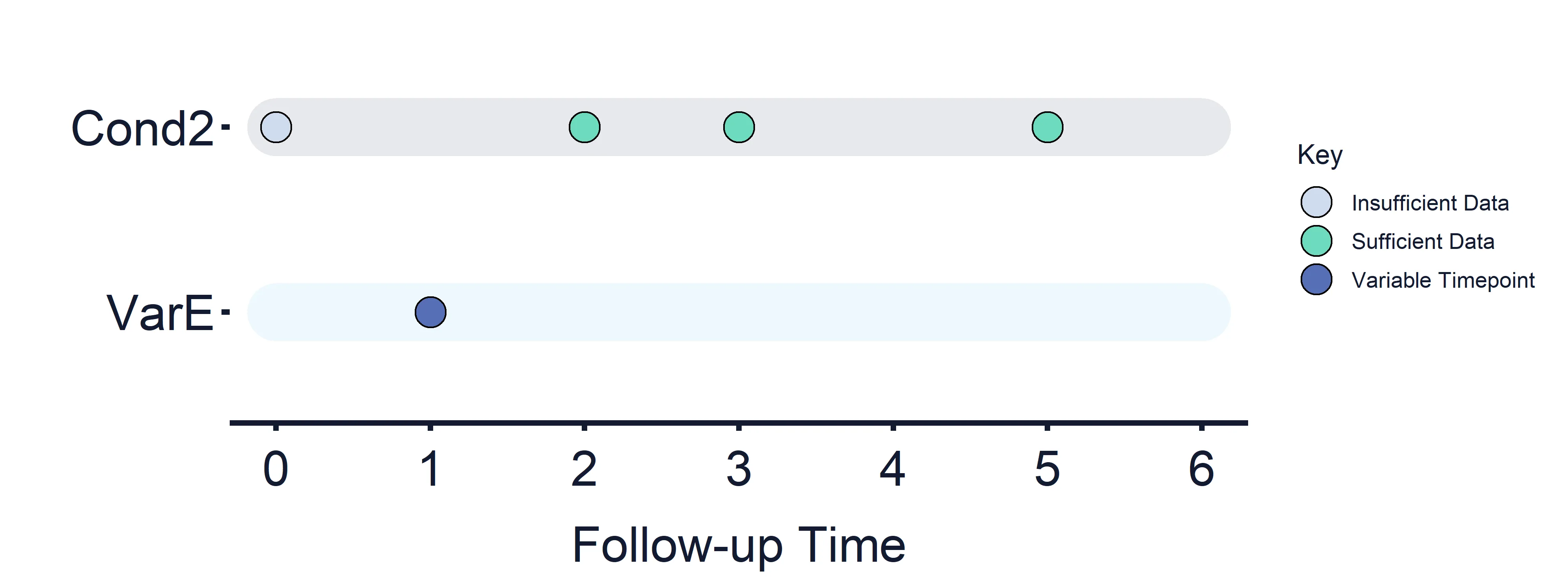Figure 10: Applying Estimand Intercurrent Event Strategies timeline.

Note

If the selected Estimand Condition is based on Variables with Timepoints, and data is not available for both the Left and Right side of the condition comparison at the timepoint of the variable to which the estimand is being applied, the condition results will default to False, as in this example.

Estimand Intercurrent Event Strategy Types

Estimand Intercurrent Event Strategies are defined by selecting one of the Replace With options described below from the dropdown menu. There are eight standard estimand replacement strategy types: Replace with Missing, Value, Variable, No Change, Maximum, Mean, Median and Minimum.

Scenario-based Estimand Strategies can be created if Estimand Scenarios have been defined for a project. Different Replace With selections can be made for each scenario in the case of scenario-based Estimand Strategies, while single Estimand Strategies are applied across all Estimand Scenarios in a project.

Replace with Missing

When the Condition for a participant is evaluated to True the estimand variable values will be treated as missing data by replacing the variable value for that participant with NA.

Replace with Value

When the Condition for a participant is evaluated to True that participant’s variable value will be replaced with a single user-specified value. To ensure valid data for analyses the replacement values that can be entered are restricted by the estimand variable type: for example, a replacement value for a Log-Normally distributed variable must be positive, and a replacement value for a Binomially distributed variable must be one of its variable levels.

Replace with Variable

When the Condition for a participant is evaluated to True that participant’s variable value will be replaced with the value of a different variable for that same participant. To ensure valid data for any analyses the replacement variables that can be selected are restricted by the variable types: for example, a replacement variable for a Poisson distributed variable must also have integer values, and a replacement variable for a categorical variable must have the same level names as the estimand variable.

Replace with No Change

Selecting “No Change” provides a way of ignoring an Intercurrent Event for an Estimand Scenario. When selected, the evaluation of the condition is skipped in the selected scenario so the following Intercurrent Events will still be evaluated for that scenario (even if the condition for the “No Change” Intercurrent Event evaluates to True). This can be used to create Estimand Definitions to consider different intercurrent events in different scenarios.

Replace with Mean/Median/Minimum/Maximum

When the Condition for a participant is evaluated to True that participant’s variable value will be replaced with a value calculated on the variable specified in the Variable dropdown. To ensure valid data for any analyses, the possible replacement variables are restricted by the variable types: for example, a replacement variable for a Poisson distributed variable must also have integer values. The Defined By selection controls across which subgroup of the population the replacement value is calculated. If “Population” is selected, then the Mean/Median/Minimum/Maximum is calculated across all participants. If “Group” is selected, then either the replacement value can be calculated for a specific subgroup (eg replace with the Mean of VarX from the control Group) or, if “Subject Identity” is chosen, a replacement value is calculated within each subgroup and the variable value replaced with the value calculated from its subgroup. For example, a participant in the control Group would be replaced with the mean of the control Group, and a participant in the treatment Group with the mean of the treatment Group. The Mean replacement strategy is not available on categorical or integer-valued variables. Replacement values calculated on categorical variables are calculated using the level values associated to variable levels or, if these are not defined, by ranking variable levels in the order that they were defined.

Applying Estimands to Repeated Measure Variables

All replacement strategy types can be applied to Continuous RM variables. The Estimand Condition results informing whether the replacement strategy should be applied will be selected on the basis of timepoint matching described previously.

If the replacement strategy depends on the values of another variable (as for Replace with Variable and Replace with Mean/Median/Minimum/Maximum) then, if the replacement variable is also a Repeated Measures variable, the replacement variable values from the corresponding timepoint will be used to calculate the new estimand variable values at each timepoint. If a timepoint was not defined for the replacement variable, then the estimand variable values will be replaced with NA if the condition is True. When the replacement variable is not a Repeated Measures variable, the values of the replacement variable are used to calculate the replacement values for all timepoints of the estimand variable.

Replace with Linear Interpolation

Linear Interpolation is available as a replacement strategy for Continuous RM variables. This replacement strategy should be used with an Estimand Condition involving a Repeated Measures variable. The Estimand Condition is evaluated at each timepoint of the estimand variable. When the condition evaluates to True for a timepoint, the corresponding variable value is replaced with a value calculated by linear interpolation across the same participant’s variable values at the preceding and following timepoints. Only values where the Estimand Condition is not True are used in the linear interpolation, and if there are no such valid values, or no preceding or following timepoints to use for interpolation, then the variable value is replaced with NA.

Replace with Carry Forward

Carry Forward is available as a replacement strategy for Continuous RM variables. This replacement strategy should be used with an Estimand Condition involving a Repeated Measures variable. The Estimand Condition is evaluated at each timepoint of the estimand variable, and when the condition is True for a participant the variable value is replaced with the value from the most recent timepoint where the Estimand Condition is not True. If no such timepoint exists, the value is replaced with NA.

Applying Estimands to Time-to-Event Variables

The only estimand replacement strategy types which can be applied to Time-to-Event variables are “No Change” and Time-to-Event-specific estimand strategy types. This is due to the structure of Time-to-Event variables which are composed of both follow-up time and whether each participant in the study had an event or were right-censored at this time.

Variable Treated as Event and Variable Treated as Censored

Variable Treated as Event and Variable Treated as Censored are available as a replacement strategies for Time-to-Event variables. These replacement strategies should be used with an Estimand Condition comparing a Time-to-Event variable with a numeric variable representing the time distribution for an intercurrent event impacting participant outcomes, such as surgery or treatment cessation. The Estimand Condition is evaluated, comparing the follow-up time for each individual with the value of this numeric variable. When the condition is True for a subject the follow-up time aspect of the Time-to-Event variable is replaced with the value from the specified replacement variable (selected from the “Replace With” dropdown menu), and the Censored aspect of the Time-to-Event variable is replaced with “Event” in the case of Variable Treated as Event and “Censored” in the case of Variable Treated as Censored.

Note

Variable Treated As Event/Censored Strategies will only be applied when the Estimand Condition result does not have Timepoints. Therefore, when creating an Estimand Condition for this Estimand Intercurrent Event Strategy, neither variable in the Variable-to-Variable comparison should have a timepoint.

Note

The same Time-to-Event variable should be used to create the Estimand Condition as the Time-to-Event variable the estimand definition is being defined for. This is because time is inherent in the Time-to-Event variables so the condition results based on an Estimand Condition with a Time-to-Event variable will be based on the time recorded for each participant as part of that Time-to-Event variable, while this time may be different for each participant for a different Time-to-Event variable. For example, each participant will have different times for Overall Survival vs Progression Free Survival.

Simulation Options

The Simulation Options consist of

1. Max Cohort Size: enter an integer between 10 and 20,000. This defines the maximum sample size that can be obtained per simulation. Within Study Design sample sizes are requested as part of the analyses framework. The Max Sample Size entered here must be bigger than the biggest sample size requested within Study Design. For further discussion see Study Design and Analysis section
2. Number Of Simulations: enter an integer between 10 and 10,000
3. RNG Seed: Random number generator seed using the internal clock to provide the starting value for the randomisation. By noting the number, it is possible to derive the exact same data every time the same seed is used, assuming that all the simulation specifications of variables and distributions stay the same too.

Random Number Generation Seed

The RNG Seed kind is “Mersenne-Twister”.

Virtual Population Review

This page provides an overview of all the set up covering the variables, their distribution and any advanced options or correlations defined. This overview allows you to verify and make any necessary changes before proceeding.

You can choose from three different speed options to run a task. After selecting a speed, the credit usage for the task will be updated, allowing you to select the option which best balances speed and cost for your needs. Find out more.

Once happy with the set up check the number of Kerus Credits which will be used and click on the Go button to generate the Virtual Population dataset which the Analyses (Study Design and Analysis) and Decision Criteria will then be based on.